The environment of the Archean Eon from 4 to 2.5 billion years ago has to be understood to appreciate biological, geological, and atmospheric evolution on our planet and Earth-like exoplanets. Its most distinguishing characteristic was negligible oxygen, unlike today’s air, which contains, by dry volume, 21% oxygen, 78% nitrogen, 0.9% argon, and 0.1% other gases. With its radically different atmosphere and lack of macroscopic, multicellular life, the Archean world was alien. However, at that time, the beginnings of modern Earth emerged. For example, Cyanobacteria probably evolved during this period, and these oxygenic photoautotrophs eventually oxygenated the air, setting the stage for later, complex life, including us.
The earliest well-preserved sedimentary and volcanic rocks are Archean and provide insights into atmospheric composition, climate, and life. These perspectives are unavailable for the Hadean eon, from about 4.6 to 4 billion years ago, which generally lacks these rocks. For context, the Archean precedes the Proterozoic eon of 2.5 billion to 541 million years ago, and Archean eras provide a timeline for Catling and Zahnle's discussion: the Eoarchean (4 to 3.6 billion years ago), Palaeoarchean (3.6 to 3.2 billion years ago), Mesoarchean (3.2 to 2.8 billion years ago), and Neoarchean (2.8 to 2.5 billion years ago).
The Archean was originally conceived to span the time from after the originof life to the advent of free oxygen. While the origin of life dates back to before 3.5 to 3.8 billion years ago or earlier, newer information puts atmospheric oxygenation after 2.4 billion year ago, inside the Proterozoic. Therefore, considering the Archean in the older sense, the origin of life falls outside this Eon, while the story of oxygen’s rise falls within.
Data about the Archean atmosphere come from how individual gases, or the air as a whole, affected chemical and physical phenomena (e.g., the composition of aerosols, chemical reactions in soils, raindrop terminal velocity, isotopic fractionations, etc.) that were recorded in rocks. So, after a brief discussion of the Hadean, Catling and Zahnle review what the Archean atmosphere was made of. However, because of limited proxy data, major uncertainties remain about the exact levels of atmospheric gases over time.
Catling and Zahnle's discussion also considers evidence for early life and its possible global influence. They assume that metabolically useful gases would have been consumed, while waste gases would have been excreted, as they are today.
Oxygenic photosynthesis produced the most impactful waste gas. The oxygen from Cyanobacterial ancestors flooded the atmosphere rapidly at a time between 2.4 and 2.3 billion years ago, with the transition marked in the rocks by the sudden disappearance of mass-independent fractionation of sulphur isotopes. The Great Oxidation Event thus began, which ended about 2.1 to 2.0 billion years ago. Although this switch to an oxygenated atmosphere and shallow ocean occurred in the Palaeoproterozoic era (2.5 to 1.6 billion years ago), the weakly reducing atmosphere that was eliminated typified the Archean. In this context, 'weakly reducing' means minor levels of reducing gases, such as carbon monoxide, hydrogen, and methane, in an anoxic atmosphere of bulk oxidized gases, carbon dioxide and nitrogen. A major outstanding question concerns how trends of biological and geological evolution relate to the Great Oxidation Event.
Atmospheric composition, in turn, affected Archean climate. At 4 billion years ago, solar luminosity was 25 to 30% lower than today, but Archean Earth was not persistently frozen because abundant evidence shows an active hydrological cycle. Liquid water under a fainter Sun likely implies more abundant greenhouse gases than today.
In addition to a gradual increase in solar luminosity, slow changes in the solid Earth over time provided boundary conditions for atmospheric evolution. On geological time scales, volcanic and metamorphic gases replenish atmospheric volatiles that escape to space or are chemically sequestered into solid materials.
The composition of the Hadean atmosphere is obscured by a lack of well-preserved rocks, but analysis of zircons, crystals of zirconium silicate, suggests that continents, oceans, and perhaps life all originated in the Hadean. Zircons are tiny (less thab 0.5 mm) durable pieces of continental crust. Elevated oxygen¹⁸/oxygen¹⁶ in 4.3-billion-year-old zircons was possibly inherited from oxygen¹⁸-enriched, weathered surface rocks that were later buried and melted, which implies the presence of surficial liquid water and even land. In addition, graphite inside a 4.1-billion-year-old zircon has a biogenic-like carbon¹³/carbon¹² ratio of −24 per mil compared to a standard reference material, although lack of context means that an abiotic origin cannot be eliminated.
Impact bombardment would have affected Hadean and subsequent Archean environments. The lunar record implies a decay of terrestrial impact bombardment extending into the Archean. The estimated median age of the last impact big enough to vaporize the entire ocean is about 4.3 billion years ago, which provides a crude upper age limit on the origin of life. An origin of life during the period 4.3 to 4.0 billion years ago is consistent with phylogenetic inferences. Later, the Late Heavy Bombardment is a hypothesized interval of enhanced bombardment superposed on the general decline, which occurred between 4.2 and 4.0 to about 3.5 billion years ago, based on the ages of lunar rocks and meteorite shocks, althoughmany dispute that the Late Heavy Bombardment was a discrete event. Regardless, an Late Heavy Bombardment would likely not sterilise Earth; any microbial life would have rebounded.
The mantle contains excess highly siderophile elements (elements that will dissolve readily in iron either as solid solutions or in the molten state, which tend to sink into the core) relative to concentrations expected after Earth’s iron core formed, which removed highly siderophile elements. Similarities of isotopes and relative proportions of these highly siderophile elements to those in enstatite chondrite and achondrite meteorites suggest that this highly reducing meteoritic material was delivered late in Earth’s accretion. Thus, carbon and nitrogen were supplied in graphite and nitrides. Therefore, the Hadean atmosphere and mantle were probably initially highly reducing, before subsequent oxidation either by hydrogen escape or disproportionation of mantle iron oxide accompanied by iron loss to the core. In any case, iron-cored impactors would reduce seawater to hydrogen and create transient, highly reducing atmospheres that may have been important for the origin of life.
Because a liquid ocean likely existed by about 4.4 billion years ago, feedbacks in the geologic carbon cycle probably stabilised the long-term climate. However, consumption of carbon dioxide in the weathering of impact ejecta by carbonic acid suggests a cool early Hadean surface near 0°C under the faint Sun.
Estimates of nitrogen bound in today’s solid Earth range a few to about 40 bar equivalent, which allows for considerable nitrogen in the Hadean atmosphere unless nitrogen was incorporated into a reducing, deep layer of magma, a magma ocean, formed after the Moon-forming impact about 4.5 billion years ago. So, although nitrogen was one of the bulk atmospheric gases, its Hadean level, higher than today or lower, remains unclear.
Precambrian events and atmospheric change. Catling & Zahnle (2020).
Proxies constrain Archean atmospheric composition. Gases reacted with the seafloor or land, leaving chemical traces in seafloor minerals or in soils that became palaeosols. In addition, atmospheric particles carried isotopic signatures into sediments that were diagnostic of atmospheric composition. Occasionally, fluid inclusions in rocks trapped seawater with dissolved air or even microbial gases.
Sometimes the physical environment affected rocks and minerals. Their preservation allows estimates of environmental temperature and barometric pressure.
The strongest constraint on Archean atmospheric composition is that the ground-level mixing ratio of oxygen was less than one millionth of present atmospheric level or less thab 0.2–parts per million by volume oxygen for air of 1 bar, indicated by the presence of sulphur isotope mass-independent fractionation in Archean sedimentary minerals. An oft-quoted limit of one hundred thousandth present atmospheric oxygen derives from an earlier photochemical model that could not address oxygen levels lower than this. Usually, isotope fractionation is proportional to the mass difference between isotopes; e.g., in diffusive separation of sulfur-containing gases, sulphur³⁴ becomes about half as abundant, relative to sulphur³², as sulphur³³. However, some particular photochemical reactions produce mass-independent fractionation that, by definition, deviates from proportionality to mass.
Archean sulphur isotope mass-independent fractionation is tied to the production of elemental sulphur from photochemistry in anoxic air; in contrast, in an oxic atmosphere, sulphur isotope mass-independent fractionation nearly disappears. Photochemistry imparts sulphur isotope mass-independent fractionation and produces elemental sulphur, starting with reactions that photolyse volcanic sulphur dioxide. This photolysis occurs when short-wavelength ultraviolet penetrates Earth’s troposphere in the absence of a stratospheric ozone layer. Scarce ozone implies negligible molecular oxygen, from which ozone derives.
In anoxic air, sulfur ends up in insoluble octasulphur aerosols and watersoluble sulphate and sulphur dioxide, unlike today’s atmospheric sulphur, which almost entirely oxidises to sulphate. In the Archean, as well as anoxia, gases such as methane or hydrogen produced sufficiently reducing conditions that sulphur gases persisted and polymerized into octasulphur. Reactions that dominantly imparted sulphur isotope mass-independent fractionation are debated: They include polysulphur formation, sulphur dioxide photolysis, and other reactions. In any case, when octasulphur particles fell to Earth’s surface, their sulphur isotope mass-independent fractionation isotopic composition complemented that of sulphate particles, allowing preservation of different sulphur isotope mass-independent fractionation signs in these phases as sedimentary pyrite (iron sulphide) and barite (barium sulphate). Sulphate, of course, could later be microbially transformed to pyrite.
Numerous redox-sensitive tracers corroborate negligible Archean oxygen. Anoxia proxies that have long been recognised include the lack of pre-Great Oxidation Event continental sediments stained by red ferric oxides (redbeds), detrital grains from well-aerated rivers of siderite (iron carbonate), uraninite (uranium dioxide), or pyrite that would oxidise and dissolve or rust at high oxygen pressures, and palaeosols with iron washed out by anoxic rainwater. Furthermore, Archean marine sediments have low concentrations of elements that enter rivers during oxidative continental weathering. Conversely, glacial sediments contain continental materials lacking oxidative weathering loss of molybdenum.
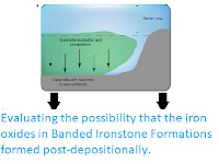
Iron formations, which are marine chemical sedimentary rocks rich in iron and silica (15 to 40 percent by weight iron and 40 to 60 percent by weight silicon dioxide), indicate that the deep Archean ocean contained aqueous (disoloved) iron and so was anoxic. In 'Superior-type iron formations' that formed near-shore, rare earth elements show that dissolved iron was partly sourced from seafloor hydrothermal vents and upwelled onto continental shelves where the iron precipitated. In today’s deeply oxygenated oceans, oxidised iron instead precipitates locally around vents. Archean shallow-water iron formations constrain atmospheric oxygen at less than 0.0024 bar.
The absence or presence ofmass-dependent fractionation of various isotopes can also indicate anoxic versus oxic conditions. In the case of sulphur, today’s oxidative weathering of continental sulphides produces soluble sulphate, which rivers carry to the ocean. When Bacteria reduce sulphate to pyrite in seafloor sediments, they impart mass-dependent sulphur isotope fractionation if sulphate is present at sufficient concentrations, as in the modern oceans, but usually not in Archean seawater. The absence of this isotope fractionation indicates little Archean seawater sulphate and implies anoxic air. Using similar arguments of oxygen-sensitive weathering, transport, and fractionation, isotopes of copper, chromium, iron, uranium, molybdenum, and selenium, indicates an anoxic Archean atmosphere.
Atmospheric oxidation of 2.7-billion-year-old iron-nickel micrometeorites has been used to argue for oxygen near-modern levels above about 75 km altitude. However, given copious evidence for an anoxic Archean atmosphere, an alternative explanation is that high carbon dioxide levels (perhaps over 70%) oxidised the micrometeorites.
Nonetheless, even under a globally anoxic atmosphere, lakes and shallow seawater inhabited by oxygenic photosynthesisers could have become 'oxygen oases', local or regional areas with elevated Oxygen, although estimates for disolved oxygen levels in Archean oxygen oases only range from 0.4 to 7% of present disolved oxygen levels in surface seawater.
When exactly oxygenic photosynthesis began and dominated over anoxygenic photosynthesis is debated, but signs of biological carbon fixation appear early. Graphite in a roughly 3.7-billion-year-old outcrop of sedimentary rock is carbon¹²-enriched in amounts typical of photosynthetic microbes. Then, at 3.52 billion years ago, the proportion of carbon¹³ in kerogen and associated marine carbonate of found in Australia is similar to biological isotope fractionation in modern oceans.
Fossil evidence for Archean Cyanobacteria has been reported. Light organic carbon isotopes and structures like those made by filamentous Cyanobacteria found within Stromatolites or other microbially induced sedimentary structures are consistent with Cyanobacteria by 3.2 to 2.7 billion years ago. Cyanobacteria could be corroborated by biomarkers, which are remnant organic molecules from particular organisms. However, putative Archean biomarkers have been plagued by younger contamination.
Instead, Cyanobacterial interpretations are strengthened by geochemical data suggesting oxygen oases at 3.2 to 3.0 billion years ago. Fractionated iron and molybdenum isotopes and levels of redox-sensitive metals suggest marine photic zone oxygen (chromium isotope data have been used to argue for the existence of approximately 3-billion-year-old terrestrial oxygen, but they were probably caused by modern oxidative weathering).
Then, by 2.8 to 2.6 billion years ago, increasing concentrations and isotopic fractionation of molybdenum and sulphur in marine shales suggest that oxygen proximal to Cyanobacterial mats and Stromatolites on land oxidised sulphides and boosted sulphate and molybdenum riverine fluxes to the oceans. These trends are consistent with isotopic evidence for Neoarchean methanotrophy and oxidative nitrogen cycling.
Concentration spikes at 2.5 to 2.66 billion years ago in molybdenum, selenium, and rhenium and isotopic excursions of molybdenum, selenium, uranium, and nitrogen have been interpreted as arising from oxygen transients or 'whiffs' of oxygen. Critics argue that the data derive from post-Great Oxidation Event alteration. Alternatively, oxygen oases of Cyanobacteria within soils or lakebeds may have mobilised these elements into rivers and then the sea.
Phylogenetic analyses mostly suggest that Cyanobacteria originated by 2.8 billion years ago. Molecular clocks must be calibrated by physical evidence, and phylogenetic methods are themselves debated. While some argue that oxygenic photosynthesis evolved only 50 to 100 million years before the Great Oxidation Event, most studies suggest an earlier Palaeoarchean or Mesoarchean age.
Amajor unresolved issue is how the Great Oxidation Event was related to underlying geological or biological trends. Life on its own cannot change the net redox state of the global environment because each biological oxidant is complemented by a reductant. In oxygenic photosynthesis, a mole of organic carbon accompanies every mole of molecular oxygen.
Consequently, for long-term molecular oxygen accumulation, some organic carbon must be segregated from the oxygen and buried. Alternatively, oxygen molecules are liberated if microbes use the organic carbon to make other reductants, such as sulphides from sulphates, that are buried. However, Archean seawater sulphate concentrations were small, so organic carbon burial is the oxyen flux that matters for the Great Oxidation Event. Atmospheric oxidation also occurs when hydrogen escapes to space after the photochemical breakdown of gases such as molecular hydrogen and methane, which ultimately derive from water and are relatively abundant in anoxic air.

Schematic history of atmospheric oxygen. Colored arrows represent known oxygen constraints, but the black line is speculative. An Archean upper bound of under 0.2-mbar oxygen (blue) is for photochemistry that generates octasulphur aerosols, preserving observed mass-independent isotope fractionation in sulphur compounds. The size and shape of an oxygen overshoot during the Great Oxidation Event are highly uncertain; a lower bound (red arrow) comes from iodine incorporation into carbonates. In the Proterozoic, a lower bound (light green) of 0.006 bar is required for an oxygen-rich atmosphere to be photochemically stable. However, oxygen levels likely remained low for most of the Proterozoic. Neoproterozoic oxygenation began around 800 million years ago. From about 600 million years ago, a lower bound of over 0.02-bar oxygen (dark green) is from plausible oxygen demands of macroscopic Ediacaran and Cambrian biota. Charcoal since 400 million years ago ago implies a lower bound of over 0.15 bar (purple). The post-Devonian black line for oxygen evolution approximately represents curves from calculations of carbon and sulphur isotopic mass balance. Catling & Zahnle (2020).
Atmospheric oxygen is determined by net redox fluxes into and out of the atmosphere. This simple truth is deceptive because these redox fluxes are themselves controlled by less easily constrained oxidative weathering (both seafloor and continental) and volcanic and metamorphic degassing, as well as hydrogen escape to space. Permanent atmospheric oxygenation requires an oxygen level of 0.03 x present atmospheric level or more to prevent a destabilising positive feedback of photochemical destruction of tropospheric oxygen that otherwise occurs when an incipient ozone column is still transparent to far ultraviolet light.
These oxygen levels would have only been attained when the oxygen flux from the burial of organic carbon exceeded the kinetically efficient sink from oxygen-consuming gases (carbon monoxide, hydrogen, hydrogen sulphide, and sulphur dioxide) from volcanism and metamorphism plus fluxes of reducing cations such as iron²⁺ from seafloor vents. A minority assume that such a flux imbalance applied as soon as oxygenic photosynthesis evolved, mandating a rapid rise of atmospheric oxygen. In the consensus assessment that oxygenic photosynthesis evolved long before the Great Oxidation Event, efficient consumption of oxygen initially suppressed oxygen levels.
Ideas favoring increased oxygen fluxes from organic burial appeal to more continental shelf area available for burial, more phosphorus to stimulate photosynthesis, or subduction of organic carbon relative to ferric iron. Because organic carbon burial extracts carbon¹² and leaves inorganic carbonates carbon¹² depleted, it is difficult to reconcile these hypotheses with the remarkable constancy of the carbon isotope record, which indicates little change in average organic burial rates between the Archean and Proterozoic. However, an increase in organic burial might have occurred if negligible oxidative weathering of carbon¹²-rich organics on land or a sink of seafloor carbonate meant that the operation of the carbon cycle or the isotopic composition of carbon input into the surface environment differed from today.
Hypotheses for a slowly decreasing oxygen sink to the Great Oxidation Event tipping point rely on a decline in the ratio of reduced-to-oxidised species from volcanic, metamorphic, and hydrothermal sources. Some emphasize the role of hydrogen escape to space in oxidising solid Earth, lowering Earth’s capacity to release oxygen-consuming reductants. New evidence from xenon isotopes supports rapid Archean hydrogen escape.
Molecular nitrogen dominates today’s atmosphere, and three lines of evidence have begun to constrain Archean nitrogen levels. First, the largest size of 2.7-billion-year-old fossil raindrop imprints provides a conservative limit of paleopressure of under 2.1 bar and a probable limit of under 0.52 to 1.2 bar. Second, the molecular nitrogen/argon³⁶ ratio in fluid inclusions indicates a nirogen presure of less than 1.0 bar at 3.3 billion years ago and less than 1.1 bar at 3.5 to 3.0 billion years ago. Third, vesicle volumes in 2.7-billion-year-old basaltic lava flows erupted at sea level imply a 0.23 bar palaeopressure.
The inferred history of nitrogen presure depends on how the geologic nitrogen cycle has changed over time. Nitrogen can only greatly accumulate as atmospheric nitrogen or in rocks as ammonium, amide, nitride, or organic nitrogen.Under typical mantle temperatures and redox conditions, volcanic gases contain molecular nitrogen, not ammonia, and because molecular nitrogen is unreactive, it enters the air. Today, molecular nitrogen is also produced when oxidative weathering of organic matter on the continents makes nitrate that undergoes rapid biological denitrification into molecular nitrogen. Within large uncertainties, volcanic and oxidative weathering inputs of atmospheric nitrogen are comparable. Using sedimentary carbon/nitrogen data, it has been argued that the sum of these nitrogen sources was balanced over the Phanerozoic primarily by nitrogen burial in organic matter, so that the Phanerozoic partial pressure of nitrogen varied little.
Another theory states that low Archean palaeopressure arose because today’s long-term nitrogen atmospheric input from oxidative weathering and denitrification was absent. If so, nitrogen presure would have risen at the Great Oxidation Event, and nitrogen in today’s air must have been in solid phases previously. Certainly on modern Earth, nitrification, by humankind’s addition of nitrate to land and sea, has enhanced denitrification, indicated by increased atmospheric nitrous oxide. On the other hand, a model can be constructed where nitrogen presure declines after the Great Oxidation Event if burial of organic nitrogen increased.
In the Hadean, nitrogen presure either started high and then diminished or was initially low if nitrogen partitioned into a very reducing magma ocean. However, low nitrogen/arbon in today’s mid-ocean ridge source basalts suggests considerable nitrogen degassing once the upper mantle became oxidised because then nitrogen became insoluble in magmas and upper mantle fluids. Even today, some of the upper mantle lies within the stability field for ammonium, so that increased oxidation of the early mantle and mantle wedge could have caused more subducted nitrogen to outgas as molecular nitrogen.
Marine phyllosilicates (sheet silicate minerals) at 3.8 billion years ago are ammonium enriched, which probably came from porewater ammonium derived from degraded organics, and these data have been used to argue that Archean nitrogen was sequestered into solid phases after an early advent of biological nitrogen fixation. In the early ocean, ammonium would have been the stable form of dissolved nitrogen unlike today’s nitrate. Consequently, a postulated drawdown of Archean nitrogen involves biological fixation, organic burial, and subduction of ammonium in refractory minerals. The rate of organic burial must have been relatively high for a time-integrated loss to affect nitrogen presure significantly, which is not necessarily inconsistent with carbon isotopic constraints because early high degassing of carbon required more carbon to be buried.
Nitrogen isotopes appear to confirm that biologically fixed nitrogen entered the Archean mantle. Sedimentary organics have 7 parts per thousand more nitrogen¹⁵ as a proportion of total nitrogen; compared to modern atmospheric nitrogen, whereas mantle nitrogan has 2 parts per thousand less nitrogen¹⁵ than modern atmospheric nitrogen. Fractionation mostly arises when denitrification preferentially converts nitrate or nitrite nitrogen¹⁴ into gaseous molecular nitrogen. Thus, heavy nitrogen¹⁵ in 3.1 to 3.5-billion-year-old mantle-derived diamonds may be a sedimentary component.
Ammonium substitutes for potassium, and breakdown of previously subducted ammonium-containing minerals in magmas at oceanic islands releases moleciular nitrogen and radiogenic Argon⁴⁰ derived from Potasium⁴⁰. The ratio Argon⁴⁰/moleciular nitrogen in plume-related lavas scatters by a factor of about 4 to 5, and higher values (older from more Argon⁴⁰) correlate with smaller, Archean-like values of nitrogen¹⁵ ratios, consistent with a history of ammonium subduction. Because moleciular nitrogen is uncorrelated with non-radiogenic Argon³⁸ or Argon³⁶, nitrogen in the current mantle is not primordial but recycled.
Some models have used nitrogen ingassing versus outgassing fluxes to infer past atmospheric nitrogen presure, however estimates of modern nitrogen outgassing vary a great deal, making such models dubious.
Unlike molecular nitrogen, other nitrogen-bearing Archean gases would have been present only in trace quantities. With only tiny atmospheric fluxes of nitrate or nitrite, nitrous oxide from denitrification would have been negligible, perhaps restricted to lakes. Lightning production of nitric oxide, followed by hydrogen addition and nitroxyl dissolution and decomposition, might maintain ground-level nitrous oxide to a few parts per billion by volume, compared to a pre-industrial levels of about 270 parts per billion nitrous oxide. The other nitrogen oxides (nitric oxide and nitrogen dioxide) would have been at trace levels because their lightning production in carbon dioxide-nitrogen air is inefficient.
Ammonia levels of 10 to 100 parts per billion would provide a greenhouse effect to counteract the faint young Sun, but these levels of ammonia cannot be sustained against ultra violet photolysis. Possibly, a stratospheric organic haze, such as that on Saturn’s moon, Titan, shielded tropospheric ammonia from ultra violet light. However, whether this shielding actually occurred depends on whether hazes actually existed and on the size and radiative properties of haze particles, which remain uncertain.
Another nitrogen-bearing gas, hydrogen cyanide is more stable photochemically than ammonia and made in reducing atmospheres by lightning, impacts, or ultra violet-driven photochemistry. In particular, nitrogen atoms from molecular nitrogen photolysis in the upper atmosphere can mix to lower levels and react with methane photolysis products to make hydrogen cyanide. At Archean biogenic methane levels of about 3000 parts per million, hydrogen cyanide concentrations reach 100 parts per million.
Since the early Hadean, carbon dioxide has probably always been Earth’s most important non-condensable greenhouse gas. Carbon dioxide also affects seawater pH and influences the carbon cycle through the formation of carbonates and organic matter. However, direct evidence for Archean carb dioxide on levels remains scanty.
Palaeosols provide some estimates. Acid leaching in Archean soils arose from carbon dioxide dissolved in rainwater. Mass-balance calculations give 10 to 50 times present atmospheric levels of carbon dioxide at 2.7 billion years ago and 8 to 69 times present atmospheric levels of carbon dioxide at billion years ago. However, these analyses assume that all the carbon dioxide that entered the soils caused dissolution, so carbon dioxide pressure could have been higher if only a fraction of the carbon dioxide had been used. Another study used an analysis with an estimate of the composition of temperature-dependent aqueous solutions during weathering and, because of a weaker dependence of weathering on carbon dioxide pressure, obtained higher carbon dioxide pressure of 85 to 510 times present atmospheric levels at 2.77 billion years ago, 78 to 2500 times present atmospheric levels at 2.75 billion years ago, and 160 to 490 times present atmospheric levels at 2.46 billion years ago.
High Archean carbon dioxide pressure does not have to induce acidic seawater and dissolve marine carbonates. Instead, an increase in calcium ion concentrations could maintain an ocean saturated in calcium carbonate at alkaline pH; alternatively, seawater pH could be slightly lower than today, but calcium carbonate would remain saturated. In fact, sedimentary marine carbonates appear from 3.52 billion years ago onward.
Calcium isotopes might provide insight into coupled Archean seawater pH and carbon dioxide pressure. These two variables and carbonate alkalinity define a system where any two variables imply the third. In evaporating seawater, calcium isotopes could undergo Rayleigh distillation (isotope fractionation) under alkaline conditions, but limestones from 2.6-billion-year-old the Campbellrand marine evaporites of South Africa show no spread in calcium isotope values, which might imply a pH of 6.4 to 7.4 for a Neoarchean sea.
Siderite (iron carbonate) in Archean iron formations has been proposed as a carbon dioxide pressure proxy if it precipitated in equilibrium with the atmosphere. However, data suggest that this siderite was diagenetic (formed within the rocks at some time after they were deposited) so Catling and Zahnle omit this proxy.
Potentially, two negative feedbacks control long-term carbon dioxide pressure. First, the net consumption of carbon dioxide in acid weathering of continents or the seafloor ends up making carbonates. Seafloor weathering occurs when water in the permeable abyssal plains dissolves basaltic minerals, releasing calcium ions and precipitating calcium carbonate in veins and pores. Second, 'reverse weathering' reactions have been proposed. This reaction consumes aqueous silicon dioxide and uses cations to make aluminosilicate clays instead of carbonates that consume carbon, so that carbon dioxide stays in the atmosphere. High dissolved seawater silica and pH are hypothesised to promote reverse weathering and create clay minerals.
If atmospheric carbon dioxide pressure is high, pH is low, and temperature is warm, the formation of carbonates is favored, and carbon dioxide pressure falls, in negative feedback on carbon dioxide pressure and climate. However, if carbon dioxide pressure is low and pH is high, reverse weathering may be an alternative to carbonate formation and a negative feedback on low carbon dioxide pressure.
Estimates of today’s reverse weathering flux vary by an order of magnitude, the rate coefficient (the rate at which a reaction occurs) for reverse weathering reactions varies by many orders of magnitude, and the solubility of authigenic phyllosilicates (needed to calculate reverse weathering) varies by over an order of magnitude. Consequently, a self-consistent, coupled carbon-silica cycle model since 4 billion years ago shows that reverse weathering can be important or unimportant for the Proterozoic climate depending on parameter choice, while reverse weathering in the Archean is muted because of the probably lower land fraction and sedimentation rate. Considering these factors, estimates of Archean carbon dioxide pressure and seawater pH that Catling and Zahnle present are based on carbonate-silicate cycle models without reverse weathering.
In the Archean, with greater seafloor production than today, seafloor weathering could have been comparable to continental weathering, and negative feedback likely maintained average Archean surface temperatures between 0° and 40°C with seawater pH 6.4 to 7.4. The corresponding carbon dioxide pressure would have been 0.006 to 0.6 bar 4 billion years ago, assuming that about 10 000 parts per million by volume methane also contributed to the greenhouse effect.
Anoxic Archean air could hold 1000 s of parts per million by volume of methane if a microbial flux of methane was comparable to today’s. Phylogenetically, methanogens date back to more than 3.5 billion years ago. In contrast, the modern oxygenated atmosphere destroys reducing gases rapidly, limiting tropospheric methane and hydrogen abundances to 1.8 and 0.55 parts per million by volume, respectively.
Evidence points to high levels of Archean methane. First, signs of methanogens and methanotrophs from light carbon isotopes in Archean organics imply methane’s presence. Second, Archean sulphur isotope mass-independent fractionation requires more than 20 parts per million by volume methane to generate particulate sulphur. Third, the deuterium-to-hydrogen ratio of 3.7-billion-year-old seawater estimated from serpentine minerals is 2.5% lighter than today, which could be explained by rapid Archean escape of hydrogen and isotopic fractionation. This hydrogen was likely derived from ultra violet photolysis of methane in the upper atmosphere. Fourth, globally extensive glaciations during the Great Oxidation Event provide circumstantial evidence for high Archean methane. At the tipping point, air flips from anoxic to oxic in only about 10 000 years, causing a roughly 10°C temperature drop by oxidizing methane. This chemical transition is far faster than the 100 000-to-1 000 000-year response of the carbonate-silicate thermostat.
Another carbon-containing gas, carbon monoxide, was probably not abundant in the presence of an Archean microbial biosphere. The Last Universal Common Ancestor was likely capable of anaerobic carbon monoxide consumption, which involves water as a substrate and catalysts such as iron sulphide that were probably widespread.With this reaction, microbes would draw carbon monoxide down to 1 to 100 parts per million by volume. However, episodic carbon monoxide levels at much higher levels may have occurred when large impacts delivered cometary carbon monoxide ice or organic matter that was oxidized.
Because of relatively abundant methane, a high-altitude Archean organic haze might have formed. This idea was first suggested in the 1980s. Empirically, if the methane-carbon dioxide ratio exceeds about 10% in an ultra violet-irradiated carbon dioxide-nitrogen-methane mixture, radicals from methane photolysis polymerise into organic particles.
When and whether an organic haze formed are uncertain. A haze could have affected tropospheric sulfur gases by blocking ultra violet photons. Consequently, the structure of sulphur isotope mass-independent fractionation variations in Archean sedimentary minerals and their correlation with light, organic carbon¹³ have been attributed to episodic hazes driven by variable atmospheric methane-carbon dioxide ratios. However, given only a hazy understanding of which species and reactions are important for sulphur isotope mass-independent fractionation, interpretations of episodic hazes are speculative rather than definitive.
The Archean lower atmosphere is unlikely to have been hydrogen-rich given the antiquity of methanogens, ome of which convert hydrogen into methane. Anoxygenic photosynthesis also consumes hydrogen. In models with methanogens and hydrogen-based photosynthesisers, atmospheric hydrogen mixing ratios depend on assumed hydrogen outgassing and biological productivity but generally are no more than 0.0001. These levels preclude hydrogen as an important Archean greenhouse gas. Detrital magnetite carried in rivers 3.0 to 2.7 billion years ago would have dissolved at high hydrogen pressures via microbial reduction of iron to its soluble form using hydrogen, providing an upper limit of atmospheric hydrogen pressure of 0.01 bar.
Changes in atmospheric xenon isotopes through the Archean stop after the Great Oxidation Event (analogous to sulphur isotope mass-independent fractionation) and potentially tell us about ancient oxygen, methane, and hydrogen levels, including in the otherwise hidden Hadean. The trend also relates to how much hydrogen escaped from Earth and hence Earth’s total oxidation over time.
Xenon in fluid inclusions in Archean rocks becomes isotopically heavier through the Archean relative to an initial solar composition until the fractionation reaches that of modern air around 2.1 to 2.0 billion years ago. Xenon dragged out into space by escaping hydrogen during the Archean and Hadean best explains the progressive mass fractionation. An alternative explanation from trapping of positively charged xenon ions in organic hazes has the problem that weathering or microbial processing of buried organics would release xenon and modulate the xenon isotopes in post-Archean air, which is not observed. Today, the nine atmospheric xenon isotopes (124 to 136) have a huge fractionation of 4.2% per atomic mass unit relative to solar or chondritic sources, whereas the six, lighter krypton isotopes (76 to 86) are barely fractionated. Earth’s xenon/krypton ratio is also 4 to 20 times less than meteorites, implying selective xenon loss.
Unlike lighter krypton, xenon is easily ionized by solar ultra violet or charge exchange with positive hydrogen ions, so positive xenon ions can be dragged out to space by escaping positive hydrogen ions. Whereas positive xenon ions are unreactive with atomic hydrogen, molecular hydrogen, or carbon dioxide, any positive krypton ions are neutralised by reactions with molecular hydrogen, explaining the lack of krypton isotope fractionation. Ions are tethered to Earth’s magnetic field lines, but a 'polar wind' of hydrogen ions escapes along open field lines at the poles, accounting for about 15% of all hydrogen that escapes today. Positive xenon ions could be dragged by a vigorous ancient polar wind. That requires copious hydrogen to be derived from relatively abundant methane and/or molecular hydrogen in the lower atmosphere. Ultra violet decomposes methane in an anoxic upper atmosphere, releasing hydrogen.
The hypothesized xenon escape works only in anoxic air, so, like sulphur isotope mass-independent fractionation, xenon isotopes record the Great Oxidation Event. Oxic air destroys molecular hydrogen and methane, making their abundances too low to supply enough hydrogen to drag along xenon. In addition, molecular would remove positive xenon ions in a resonant charge exchange reaction; the oxygen molecule can donate an electron to the xenon ion, creating a positively charged oxygen molecule and a xenon atom (electrons have a negative charge).
Catling and Zahnle's preliminary model finds that xenon can escape when the total hydrogen mixing ratio exceeds about 1% for the solar extreme ultra violet flux expected around 3.5 billion years ago. If nearly all Archean hydrogen was biologically converted into methane, Catling and Zahnle we interpret the xenon escape constraint of more than 1% of the hydrogen mixing ratio to be more than 0.5% methane, which is a rare empirical constraint on Archean methane.
The inferred escape of a strong reductant, hydrogen, would oxidise the entire Earth. The total oxidation during the Archean is equivalent to oxygen from a tenth of more of an ocean.
Sulphur isotope mass-independent fractionation proves that Archean sulphur-containing gases existed but tells us little about their concentrations. All sulphur gases apart from octasulphur, which condenses, are susceptible to ultra violet photolysis and are short lived and interconverting. Consequently, atmospheric sulphur is sequestered into stable sulphuric acid aerosols by oxidation or octasulphur aerosols by reduction. For a wide range of Archean atmospheric redox conditions, both types of aerosol should form and precipitate.
Although sulfur gases absorb ultra violet, they probably did not shield Earth’s surface. Surface temperatures greater than 50°C would be required to produce enough atmospheric octasulphur vapour to shield surface life from ultra violet radiation.
Related to atmospheric composition, is another basic problem: How the Archean climate remained clement under a fainter Sun. In the Sun’s core, nuclear reactions fuse four protons into helium nuclei, increasing the mean molecularmass and decreasing the number of particles per unit volume. In response, the weight of the overlying column presses inward, and the core temperature rises. A greater radial temperature gradient drives more outward radiation flux, so the Sun brightens. Solar evolution models show that the Sun was 25 to 30% fainter at 4 billion years ago.
One solution to the Faint Young Sun problem is that the young Sun was not faint but more massive and therefore as bright as today. The Sun would then need to lose enough mass over time so that a declining weight of the column above the core matched the pressure loss from particles fused in the core. However, observations are unsupportive: Fast mass loss only happens in the first 200 million years after Sun-like stars form.
As well as solar luminosity, Earth’s mean global temperature depends on the Bond albedo (the reflectivity over all wavelengths) and greenhouse effect. Some Faint Young Sun hypotheses invoke clouds: that the Archean Bond albedo was low because of substantially different cloud cover or that abundant high-altitude cirrus clouds warmed early Earth. However, no plausible combination of few low clouds (which tend to reflect sunlight) and many high, icy clouds (which tend to warm the surface with downwelling infrared) solves the Faint Young Sun problem. Three-dimensional climate models with a lower solar flux produce weaker evaporation and fewer low clouds, but a strong greenhouse effect is still required because the albedo decrease is small.
The most plausible solution to the Faint Young Sun is a big greenhouse effect. Water vapor is an important greenhouse gas but, on its own, cannot solve the Faint Young Sun problem. Water vapor condenses into rain and snow, so its abundance is limited by the saturation vapour pressure that depends only on temperature, which is set by non-condensable greenhouse gases, such as carbon dioxide and methane.
Consequently, substantial carbon dioxide is the most obvious driver of an enhanced Archean greenhouse effect. Catling and Zahnle expect Archean carbon dioxide pressure to have been high because of Earth’s carbonate-silicate cycle thermostat. If global temperatures and carbon dioxide are low, carbon dioxide removal via rainfall is slow, as are rates of continental and seafloor silicate weathering. Then, geological emissions of carbon dioxide raise atmospheric carbon dioxide levels, increasing global temperatures. Conversely, if the climate warms too much, greater rainfall and silicate weathering consume carbon dioxide and cool the Earth.
These negative feedbacks would have moderated the Archean climate to amean global temperature of 0° to 40°C (or 0° to 50°C without land and only seafloor weathering), carbon dioxide alone could have solved the Faint Young Sun problemwith 0.004 to 0.03 bar carbon dioxide at 2.5 billion years ago and 0.024 to 1 bar carbon dioxide at 4 billion years ago, where the spread comes from uncertain carbonate-silicate model parameters.
However, without oxygen in the atmosphere, a methane greenhouse bears consideration. Methane levels of 103 to 104 parts per million by volume produce roughly 10° to 15°C of Archean greenhouse warming, which lowers the carbon dioxicde pressure needed to warm the Archean Earth. Some of this warming comes from a few parts per million by volume of ethane, which is derived from methane.
Both substantial methane and carbon dioxide may be necessary if lower bounds on nitrogen pressure are valid. Although nitrogen itself is not an effective greenhouse gas, it pressure broadens line and continuum infrared absorption, enhancing the greenhouse effect. If Archean nitrogen pressure was about half of today, a few degrees would be lost from the greenhouse effect.
However, too much methane relative to carbon dioxide would create the high altitude organic haze, which may cool Earth by up about 20°C by absorbing incoming solar radiation and radiating energy back to space in a so-called 'anti-greenhouse effect'. A cooling limit exists because as a haze becomes more ultra violet absorbing, it shields methane molecules from the photolysis needed for further haze formation. Thus, attenuation of sunlight saturates.
An organic haze might protect tropospheric ammonia from ultra violet, but whether ammonia was a viable greenhouse gas is unclear. The composition of organic aerosols in the Archean where sulphur was present and the carbon/oxygen ratio was less than 1 was different from particles on Titan where sulphur is absent and the carbon/oxygen ratio is more than 1. Consequently, the ultra violet attenuation properties of early Earth haze particles remain uncertain.
Another proposed early greenhouse gas is molecular hydrogen, if it attained percentage abundances. Molecular collisions produce temporary charge separation, allowing hydrogen to undergo collision-induced absorption of infrared photons. Archean hydrogen is unlikely to have been abundant. Instead, hydrogen may be relevant for the Hadean greenhouse, if percentage hydrogen levels arose from hydrogen outgassing or impacts.
Sulphur gases were likely unimportant for warming. Sulphur dioxide is a strong greenhouse gas, but tropospheric sulphur dioxide dissolves in rainwater, and Archean stratospheric sulphur dioxide photochemically disproportionates into ultra violet-stable polysulphur and sulphuric acid aerosols. The latter raises the albedo and more than offsets any sulphur dioxide greenhouse warming. Hydrogen sulphide is a weak greenhouse gas that overlaps in the absorption with of methane and is ultra violet fragile. Carbonyl sulphide has been suggested as an Archean greenhouse gas because ultra violet photolysis of carbonyl sulphide was posited to explain observed relationships in sulphur isotope mass-independent fractionation. Carbonyl sulphide persists today because it is not oxidised by hydroxide radicals that cleanse the troposphere of other pollutants. However, in the absence of an ozone shield, carbonyl sulphide is susceptible to photolysis and cannot build up significantly.
Last, an alternative to the carbonate-silicate cycle stabilisation of Earth’s climate is the 'Gaia hypothesis', which proposes that life interacts with inorganic Earth as a self-stabilising system that maintains habitable conditions. The Archean biosphere was surely important for atmospheric composition, which intertwines Earth’s inhabitance and habitability. However, debate continues about if and how adaptive evolution of the biosphere can produce a more stable climate than an abiotic Earth.
Catling and Zahnle next consider proxy data for the Archean climate. Glacial rocks are one line of evidence. These include dropstones in sediments from melted icebergs, unsorted clasts mixed with silt and clay deposited at the base of glaciers that are preserved as diamictites, and striations made by rocks embedded in moving glaciers that scoured underlying surfaces. In the Archean, any indication of polar environments from glacial rocks would suggest a relatively cool world given that since about 34 million years ago, a climate with poles covered in ice has required average global temperatures below about 20°C.
Glacial rocks are reported from 3.5, 2.9, and 2.7 billion years ago. The oldest, from the Barberton of South Africa, includes clasts in finely laminated sediments, interpreted as dropstones, found below diamictites. Later, in the rounghly 2.9-billion-year-old Pongola in South Africa, which was 43° to 48° palaeolatitude, diamictites contain striated clasts, while associated silty laminates have dropstones with splash-up of substrata. Then, at 2.7 billion years ago, diamictites with dropstones occur in India, and Montana.
Another line of evidence about palaeotemperature are ratios of oxygen¹⁸/oxygen¹⁶ in marine cherts and carbonates. These ratios decline with increasing age, which, at face value, suggests Archean ocean temperatures of 50° to 85°C. Cherts and carbonates precipitated from seawater acquire less oxygen¹⁸ relative to the seawater as temperature increases because, at equilibrium, warmth allows stronger oxygen¹⁸ bonds to be broken and replaced with oxygen¹⁶. Not all Archean isotopic studies infer hot temperatures, however.Combined oxygen and hydrogen isotope ratios have suggested surface temperatures below 40°C, while oxygen isotopes in Archean phosphates have produced 26° to 35°C upper limits.
Most researchers have doubted the isotopic inferences of persistently high Archean surface temperatures because the climate was sometimes cold enough for the aforementioned glaciations, and chemical weathering of quartz from hot climates is lacking. Two alternative interpretations are as follows: (i) Archean surface temperatures were similar to today’s because the oxygen isotope composition of seawater, increased by about 15 parts per thousand oxygen¹⁸ since 3.5 billion years ago. (ii) Older cherts and carbonates have nonprimary oxygen¹⁸ proportions from high alteration temperatures or hydrothermal fluids.
The first explanation relies on changes in the relative rates of high and low temperature water-rock interactions. Hydrothermal seafloor interactions increase the proportion of oxygen¹⁸ in seawater, whereas low-temperature seafloor and continental weathering decrease the proportion of oxygen¹⁸ in seawater. Archean oceans with shallow seafloor hydrothermal circulation and an increase in Phanerozoic pelagic sediments that lowers seafloor weathering might cause secular increase in the proportion of oxygen¹⁸ in seawater. However, measurements find the ancient proportion of oxygen¹⁸ in seawater matches Vienna standard mean ocean water in 2-billion-year-old ophiolites, 3.8-billion-year-old serpentine minerals, Archean pillow basalts, and kerogens in Archean cherts. In addition, clumped isotopes show little change in Phanerozoic proportions of oxygen¹⁸ in seawater. Oxygen isotopes in iron oxides since 2 billion yeasr ago suggest a secular increase in the proportion of oxygen¹⁸ in seawater.
The second possibility is that proportion of oxygen¹⁸ in cherts and carbonates is more altered with age. Microanalysis shows how chert replaced sedimentary carbonates and did not precipitate from seawater. In addition, stringent geochemical and petrographic selection criteria for palaeothermometry eliminate Archean cherts. The same issue applies for silicon isotopes in Archean cherts, which have been used to infer hot surface temperatures. Last, the triple oxygen isotope composition of Archean cherts cannot be reconciled with equilibrium precipitation from seawater and requires alteration.
Phylogenetic inferences of early thermophilic microbes have also been used to argue for hot Archean oceans However, other more convincing reconstructions and biochemical considerations suggest a mesophilic (living at below 50°C) common ancestor.
Temperature limits on mineral formation may also favor a temperate Palaeoarchean. Pseudomorphs of barite after gypsum are reported in 3.5-billion-year-old evaporites that are now partially silicified. In halitesaturated brines, gypsum forms at under 18°C; otherwise, anhydrite precipitates. It has been claimed from x-ray tomography that hydrothermal barite, not gypsum, was actually primary. However, three-dimensional universal stage petrography found interfacial angles diagnostic of gypsum at the original crystal faces, which are partially replaced by quartz and draped by quartz, and so cannot show up in x-ray density contrasts.
Additional factorsmay have affected the Archean climate. One external parameter was a faster rotation of early Earth. Today, the Moon recedes about 4 cm a year from Earth due to tides, so Earth is despinning over time to conserve angularmomentum in the Earth-Moon system.Going back in time, depositional cycles in the 2.45-billion-year-old banded iron Weeli Wolli Formation, Australia indicate a roughly 17 hour day.
In general, a faster Archean rotation rate reduces heat transport from equator to pole, particularly if the atmosphere had less mass. Thus,warm tropics and glaciated poleswould arise if the Archean
had a thin atmosphere.
External parameters that modulate the carbonate-silicate cycle would also affect the long-term climate. These include land fraction, carbon dioxide outgassing, and biological modification of weathering. In general, how carbon dioxide outgassing changedwith time dominates the uncertainty.
The general view that emerges is an Archean atmosphere devoid of oxygen and enriched in carbon dioxide and methane greenhouse gases that countered the Faint Young Sun. Nitrogen was a bulk gas, but proxy data, although debated, suggest that nitrogen levels were similar to today or possibly a factor of a few lower, which, if correct, requires understanding of how the nitrogen cycle operated differently in an anoxic world.

An overview of post-Archean atmospheric evolution in the context of biological evolution and constraints on mean global temperature in the Archean in the context of the glacial record. (A) Uncertainties on gas concentrations are a factor of a few or more. Atmospheric nitrogen may have tracked oxygen levels due to an oxidative weathering and denitrification source of nitrogen, but nitrogen pressure changes are debated. Methane was oxidized as oxygen rose but could have been protected subsequently under an ozone layer, depending on post-Archean methane source fluxes. The secular decline of carbon dioxide is a feedback effect in the geological carbon cycle induced by decreasing solar luminosity. (B) Constraints on Archean mean global temperature. Vertical blue bars denote that glacial rocks exist, noting that the durations of glaciations in the early Proterozoic and earlier are poorly known. A proposed Mesoproterozoic glaciation is not plotted because its age is disputed and possibly Sturtian. Cainozoic glaciations only occur at a global mean temperature below about 20°C. Red arrows on the Archean glaciations are a more conservative 25°C upper limit, taking into account of the possible effects of different land configurations and lack of vegetation. Low carbon dioxide during the Phanerozoic (A) correlates with glaciations (B), such as the Carboniferous-Permian ones, 335 to 256 million years ago. Precambrian greenhouse gasesmust also have fluctuated, but the amount is unknown and so not reflected in (A). Catling & Zahnle (2020).
The Archean climate was probably mostly moderate. Although some argue for a hot Archean climate, glacial rocks at 2.7, 2.9, and 3.5 billion years ago and recent isotopic analyses call that idea into question; indeed, our current understanding of feedbacks in the geologic carbon cycle suggests surface temperatures within 0° to 40°C.
Reconstructing the history of oxygen is informed by proxies, but they are often indirect. Once cyanobacteria evolved, local or regional oxygen oases in lakes or shallow seawater are possible, and various redox-sensitive proxies suggest that these oases actually existed by 3.2 to 2.8 billion years ago under globally anoxic air. The newest relevant data are mass fractionations of xenon isotopes, which gradually increase through the Archean relative to initial solar values. These data are best explained by xenon escaping to space as an ion dragged out by hydrogen originating photolytically from an anoxic atmosphere enriched in methane until the Great Oxidation Event.
Despite improved knowledge of theArchean, a relative dearth of uncontested data that constrain basic environmental variables, such as Archean seawater pH, climatic temperature, barometric pressure, and changing levels of the greenhouse gases carbon dioxide and methane through time, means that more proxy development and measurements are critical. It is also implausible that the Archean, one-third of the history of Earth, had a constant climate. However, our knowledge of Archean climatic variability is meager.
The biosphere was surely a major influence on Archean atmospheric composition, as it is today. Consequently, resolving when key biological innovations evolved, such as nitrogen fixation, methanogenesis, anoxygenic photosynthesis, and oxygenic photosynthesis, and understanding their influence are essential for improving models of atmospheric evolution.
This understanding may help us interpret future exoplanet data because atmospheres on other rocky Earth-sized worlds would initially be anoxic. On Earth, oxygenic photosynthesis evolved only once, perhaps because of its biochemical complexity. Consequently, if life exists elsewhere, inhabited planets with Archean-like atmospheres may be the most common type. So, determining what the Archean atmosphere was made of, and the influence of life, could help us distinguish biogenic gases in exoplanet atmospheres and so find life elsewhere.
Finally, the connection between atmospheric evolution and debated trends in solid Earth evolution was outside the scope of Catling and Zahnle's review. However, quantifying temporal changes in land area, surface rock composition, weathering, the size of volcanic and metamorphic fluxes of gases, and the redox evolution of outgassing all need further development to understand their implications for Earth’s atmospheric evolution or to extrapolate to exoplanets.
See also...