Evidence for life in the clouds of Venus.

Venus resembles the Earth in many ways; it is roughly the same size, giving it similar gravity, which in turn enables it to retain a thick atmosphere, something the other rocky planets of the Solar System (Mercury and Mars) lack. Unfortunately, the atmosphere of Venus is a little bit too dense for this model to carry any further; Venus is shrouded in a dense cloak of carbon dioxide, resulting in a runaway greenhouse effect and a surface temperature of about 700K (427°C). Despite this apparent hostility, scientists have long speculated that life might exist on Venus, not on its surface, but in the cloud layer between 48 and 60 km above, where Earth-like temperatures and pressures prevail.

 

The planet Venus as imaged by the Mariner 10 space probe in 1974. NASA/JPL/Caltech.

Venus has a layer of clouds about 20 km thick, including the 12 km which have Earth-like, temperate conditions. Unfortunately, these clouds are thought to be made not of of water droplets, but concentrated sulphuric acid, with a very low water content, quite unsuitable for any form of life as we understand it. 

However, 50 years of spectrographic observations of Venus have left a number of unresolved mysteries about the planet's atmosphere. 

The most puzzling of these is the presence of water and sulphur dioxide in the atmosphere above the clouds. Water is present throughout the atmosphere of Venus, albeit at very low levels, while sulphur dioxide, which can be measured in parts per million below the clouds, can still be measured in parts per billion above the clouds. Both gasses are thought to be present in the atmosphere of Venus as a result of volcanic emissions, and should in theory be uniformly mixed throughout the atmosphere to an altitude of about 70 km, where they should be destroyed by ultraviolet photodissociation. However, the observed abundances do not support this, suggesting that sulphur dioxide is significantly depleted relative to oxygen in and above the cloud layers.

Previous models have suggested that sulphur dioxide could be photochemically oxidized to sulphur trioxide, which would in turn react with water droplets in the clouds to form sulphuric acid. However, sulphur dioxide is about five times as abundant as water, so if this were happening then all water should be eliminated in the cloud layer, while the sulphur dioxide level should only be reduced by about 20%.

Another persistent mystery is the presence of free oxygen in the clouds of Venus, the formation of which cannot be explained by any current model of the planet's atmosphere and processes. Furthermore, the atmosphere of Venus appears to be in a state of chemical disequilibrium (i.e. it contains gasses that should react with one-another till one or more is eliminated unless they are being constantly being topped up).

Another mystery is the apparent presence of ammonia in Venus's atmosphere. This was first detected by the Russian Venera 8 probe in 1972, although this was initially rejected as an anomaly, but later found again by NASA's Pioneer Venus probe. Pioneer Venus's long-term observation of the clouds of Venus also found further chemical disequilibrium within the cloud layers, as well suggesting that at least the lower layers contained substantial solid material, incompatible with a sulphuric acid composition. Other mysteries uncovered within the cloud layer were the presence of methane and phosphine, as well as an unknown ultraviolet-absorbing molecule.

In a paper published in the Planetary Science Journal on 23 July 2021, Paul Rimmer of the Department of Earth Sciences and Cavendish Laboratory at the University of Cambridge, and the MRC Laboratory of Molecular Biology, Sean Jordan and Tereza Constantinou of the Institute of Astronomy at the University of Cambridge, Peter Woitke of the School of Physics & Astronomy and Centre for Exoplanet Science at the University of St Andrews, Oliver Shorttle of the Department of Earth Sciences and Institute of Astronomy at the University of Cambridge, Richard Hobbs also of the Institute of Astronomy at the University of Cambridge, and Alessia Paschodimas of the Centre for Exoplanet Science and School of Earth and Environmental Sciences at the University of St Andrews, proposed a model in which a base molecule was present in the clouds of Venus, reacting with sulphur dioxide in the atmosphere to form sulphites, and thereby explaining the depletion of sulphur dioxide in the planet's atmosphere.

This reaction would also consume water, but this would be released again as the sulphites broke down in the lower atmosphere, providing a model that would account for the observed levels of water and sulphur dioxide in the atmosphere of Venus. The formation of sulphites would also have a profound impact on the composition, and pH, of the cloud layer. This has previously been assumed to more-or-less pure sulphuric acid, resulting in a pH of about -11, but Rimmer et al.'s model would raise this to somewhere between -1 and 1. This is within the tolerance range of extremophilic Bacteria and Archaeans on Earth, whereas -11 would be completely unsurvivable for any Earthlife-like organism.

In their initial paper, Rimmer et al. used sodium hydroxide as base in their model, not because they thought it was likely to be present, but simply as a standard base with predictable interactions. In a second paper published in the Proceedings of the National Academy of Sciences of the United States of America on 20 December 2021, William Bains of the Department of Earth, Atmospheric, and Planetary Sciences at the Massachusetts Institute of Technology and the School of Physics & Astronomy at Cardiff University, Janusz Petkowski, also of the Department of Earth, Atmospheric, and Planetary Sciences at the Massachusetts Institute of Technology, Paul Rimmer, lead author of the original study, and Sara Seager, again of the Department of Earth, Atmospheric, and Planetary Sciences, and of the Department of Physics and the Department of Aeronautics and Astronautics at the Massachusetts Institute of Technology, suggest that ammonia might be the base present in the clouds of Venus, discuss the implications of that.

The presence of ammonia in the clouds of Venus would result in the observed gas balance, with the upper atmosphere depleted in sulphur dioxide, but still containing water, as well as solid particles being formed in the clouds, and the presence of free oxygen.

In order for ammonia to form in the clouds of Venus, it would be necessary to reduce nitrogen by bonding it to hydrogen, which would require source of electrons as well as a source of hydrogen. Since there is almost no free hydrogen in the clouds, Bains et al. consider water to be the most likely candidate for the hydrogen doner, with electrons being obtained by the oxidation of carbon monoxide, carbonyl sulphide, sulphur dioxide, nitrogen, water, or hydrochloric acid.

Bains et al. reason that the most likely process would be the reaction of nitrogen with water to produce ammonium hydroxide and oxygen, as this requires less water and less energy than other potential reactions, and because it is the only reaction that would directly produce both ammonia and oxygen (which have been observed) without producing other oxidized species (which have not been observed) and would then require more energy to break down releasing oxygen.

The next question Bains et al. address is the rate at which the clouds must be depleting sulphur dioxide from the atmosphere in order to produce the observed levels, assuming that the sulphur dioxide rate is being topped up from below at a steady rate. This leads to the calculation that 100 billion tonnes of ammonia must be produced each year, roughly equivalent to the amount of free oxygen produced by photosynthesis each year. This would also result in about 100 billion tonnes of mass being lost from the bottom of the cloud layer through the precipitation of solid sulphite particles, which is in line with observations.

Any reaction producing ammonia on Venus would require considerable energetic input, leading Bains et al. to look for plausible sources of such energy. Lightning is present on Venus, and is capable of reducing nitrogen to ammonia, but the level of energy available from lightning would be far short of that needed to produce the observed gas ratios, and in any case unlikely to produce free oxygen. Ultraviolet-driven photochemistry can also produce ammonia, but again is most unlikely to do so at the observed levels (although how the presence of large amounts of sulphuric acid would have on this process has never been explored). Similarly, volcanoes can produce ammonia on Earth, but it is highly unlikely that Venusian volcanoes could be producing the observed levels of ammonia.

The ability to harvest chemical energy to reduce nitrogen to ammonia in an oxidising environment is a characteristic of life on Earth, where many Microorganisms live by doing just that, so Bains et al. posit that it is not unreasonable to suggest similar organisms might be carrying out this process in the clouds of Venus. The energy requirements of such a process would be high, and there would need to be clear benefits involved for any organism to do this, but Bains et al. suggest that creating a habitable environment by de-acidifying the cloud droplets would satisfy this requirement.

 

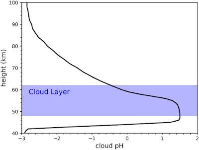
Predicted pH profile of cloud particles. The blue shaded region shows the altitude where clouds are present, from 48 km to 62 km. Note that the plot extends above and below the cloud tops because there are plausibly cloud particle populations that extend down to the altitude where sulphuric acid is sublimated, and up into the mesosphere where sulphuric acid aerosol evaporation may explain the anomalous sulphur dioxide inversion at 80 km to 100 km. This model provides no constraints on the composition of the mesospheric particles, which may well be composed of pure sulphuric acid. Bains et al. (2021).

Bains et al. suggest that the production of the levels of ammonia needed to drive this process is not beyond the plausible range of biological organisms living within the clouds. 100 billion tonnes of ammonia production per year equates to 3.10 billion grams of ammonia per second. On Earth, several species of Cyanobacteria can fix nitrogen into ammonia at rates of 0.000 000 041 g per gram of wet weight per second, which means that 8.1 billion tonnes, wet weight, of these organisms could produce 100 billion tonnes of ammonia per year. Any life in the clouds of Venus is unlikely to closely resemble Earthly Cyanobacteria, but assuming an organism with similar productivity was involved, then it would only represent about 1.5% of the mass of the lowest 5 km of the cloud layer.

Bains et al.'s model provides a better match for the observed abundances of gasses in the atmosphere of Venus, and in particular can account for; (1) the observed disequilibria in the clouds of Venus, (2) the observed presence of oxygen in the clouds, (3) the observed abundance of water in the clouds, (4) the detected ammonia in the clouds, and (5) the observed abundance profile of sulphur dioxide in and above the cloud layer.

Oxygen was detected in the clouds of Venus by the Pioneer Venus and Venera 14 probes, but this was rejected at the time due to the implied disequilibria that would have to exist in Venus's atmosphere. However, since that time is has become overwhelmingly clear that something is causing a disequilibrium in the atmosphere of Venus, and it is therefore reasonable to assume that oxygen is present. Bains et al.'s model predicts the presence of oxygen at levels at only one twentieth of the levels observed by Pioneer Venus and Venera 14 (although it does not rule out the production of further oxygen by other biological processes), but at a far higher level than any other model currently available.

Ammonia was also observed in the clouds of Venus by the Pioneer Venus and Venera 8, but this finding was also rejected at the time, as it was assumed the clouds were made up of droplets of concentrated sulphuric acid, and environment in which ammonia could not survive. Bains et al.'s model produces a much less acidic cloud layer, potentially with a pH above zero, within which ammonia could potentially exist.

Bains et al.'s model predicts the precipitation of ammonium sulphate and ammonium sulphite beneath the cloud layer, forming droplets that would fall until they are evaporated by the rising temperature of the atmosphere. This would result in the thermal decomposition of these molecules, which would release free ammonia, which would be oxidised to form nitrous oxides, something else detected by Pioneer Venus.

This model would also result in larger, probably non-spherical, droplets within the lower cloud layer, which would present a potential home for any biological organism. This is consistent with observations of the cloud layers on Venus, which again cannot easily be explained by any non-biological process.

Bain's et al.'s model can also explain the 'stagnant haze' that has been observed beneath the cloud layer on Venus. This haze extends downwards from the cloud base at 47 km above the ground, to an altitude of about 30 km, and its composition is unclear. The temperature of this haze layer is about 100°C at its upper extent and about 200°C at its base. This would be consistent with sulphate and sulphite salt particles falling from liquid droplets that evaporate at about 100°C, and which themselves decompose at temperatures of 200°C. This would also result in the formation of hydrogen sulphide in the layer beneath the clouds, something else which has been tentatively identified in the data from the Venera 14 and Pioneer Venus probes.

This study provides a new perspective on the habitability of the clouds of Venus. These clouds have previously been viewed as made up entirely of sulphuric acid, creating an extremely acidic and extremely dry environment, something deeply hostile to even the most tolerant forms of life. Bains et al.'s model shows how living organisms could inhabit a layer in the lower parts of these clouds, maintaining a much less acidic environment, with larger semisolid ammonium sulphite and sulphate particles through the production of ammonium.

The predicted pH within this layer, -1 to 1, is within the tolerance levels of some Extremophilic micro-organisms on Earth, and the temperature range, 60-80°C, is that which would be considered optimal for many such organisms. Furthermore, many micro-organisms which we would not considered extremophilic can produce ammonia as a defence against acidic conditions (including some pathogens, such as Mycobacterium tuberculosis and Candida albicans, which use this ability to neutralise the acids in phagosomes produced by our bodies as a defence against them).

Bains et al. note that there are still problems with their model. Most notably, the model only predicts a relative humidity of 0.02% in the lower cloud layer. This is 50 times drier than the lowest conditions that can be endured by the most drought-tolerant organisms on Earth (spores, and aestivating stages of Tardigrades and some micro-organisms can survive such conditions, but are not biochemically active). However, the levels of water reported in studies of the cloud layer is variable, which may mean that the distribution of water within these clouds is variable, with both arid and humid regions, allowing for the presence of active life.

The origin of life on Venus is an interesting question. Some models of Venus's history suggest that the young planet was much more hospitable, with a temperate climate and liquid water on its surface, with hostile conditions developing later due to a runaway greenhouse effect. Under such a model, life could have originated on the surface of Venus, and subsequently migrated into the clouds (this is not unreasonable as, although it is not obvious, there is quite a bit of life in the Earth's upper atmosphere).

See also...

Follow Sciency Thoughts on Facebook.

Follow Sciency Thoughts on Twitter.

 

The ability of the tropical seasonal forests of southeastern Brazil to absorb atmospheric carbon may be under threat.

Tropical forests have a key role in the global carbon dynamics by accounting for one-third of the terrestrial gross primary production and one-half of the terrestrial stored carbon. Increasing atmospheric carbon dioxide concentration, rising temperatures, drought events, and deforestation are expected to affect ecosystem functioning through plant physiological responses and forest loss over the coming decades. How tropical forests will respond to increasing atmospheric carbon dioxide concentration and climate change are sources of uncertainty in predicting their future carbon stocks and net primary productivity. Among tropical forests, the ones under stressful conditions, such as the seasonally dry tropical forests that endure periodic droughts, can be vulnerable to these environmental changes because they are already at the edge of climate niches to sustain forest formations with high biomass. Brazil has been the largest source of carbon emissions from gross deforestation up to 2013: In 2013 alone, 192 000 hectares (1920 km²) of Caatinga forests (where the largest continuous extent of neotropical seasonally dry tropical forests is located) and 24 000 hectares (240 km²) of Atlantic forests were deforested. An aggravating factor is that only 6.2% of Brazilian seasonally dry tropical forests extent is protected. In this context, it is crucial to advance our understanding of the carbon sink of these forests.

Over recent decades, the terrestrial carbon sink has been increasing globally. This phenomenon is possibly explained by the increases in atmospheric carbon dioxide concentration (carbon dioxide fertilisation), which is expected to enhance plant growth. Carbon dioxide has a key role in photosynthesis and can potentially increase water use efficiency by reducing stomata conductance. In this context, the increases in atmospheric carbon dioxide concentration are thought to have enhanced photosynthesis more than rising temperatures have enhanced respiration. Hence, drought-related stress on plant growth would be understated by rising atmospheric carbon dioxide concentration. However, the mechanisms involved in the feedbacks among vegetation, atmospheric carbon dioxide, and climate are complex. For example, the increase in photosynthesis and water use efficiency led by rising atmospheric carbon dioxide concentration does not necessarily promote stand growth because of the effects of other co-occurring factors. The effects of increasing drought, rising temperatures, competition, and physiological acclimation to higher levels of carbon dioxide can constrain tree growth and also lead to tree mortality. Therefore, it is difficult to disentangle the effects of climate fluctuations and rising carbon dioxide on carbon dynamics because these factors covary and can interact over time.

While recent studies have shown a long-term decline in the Amazon rainforest carbon sink, mostly driven by climate-induced tree mortality, others have predicted that tropical rainforest carbon sink may be resilient to climate change in the next decades. However, it remains uncertain how Brazilian seasonal forests (which are already exposed to drought), such as deciduous forests and semideciduous forests, have responded to the increasing levels of atmospheric carbon dioxide and climate fluctuations over time.

In a paper published in the journal Science Advances on 18 December 2020, a team of scientists led by Vinícius Andrade Maia of the Departamento de Ciências Florestais at the Universidade Federal de Lavras, assess how these forests are behaving over time by using long-term seasonal forest census data from southeastern Brazil to investigate the long-term trends of carbon stocks, gains, losses, and net carbon sink.

Maia et al. draw their inferences from 95 census intervals nested within 32 sites, ranging between 1987 and 2020 (mean site total monitoring length, about 15 years). The spatial (number of sites and sampled area) and temporal (interval length and total monitoring time) sampling efforts varied among sites and forest types. The forest sites used are in advanced successional stages, free from fire, flood, landslides, and Human disturbances at least for decades before the first census of each site. The data encompass a wide environmental space and three forest types (deciduous, evergreen, and semideciduous forests), allowing Maia et al. to investigate whether forests under different climates have differed in their long-term trends. In addition to the rising atmospheric carbon dioxide concentration (parts per million) and carbon dioxide change (parts per million per year) over time, mean annual temperature and mean annual precipitation have shown an unstable temporal trend in their data. Therefore, Maia et al. used time (year) as a proxy of the effects of rising carbon dioxide, climate fluctuations, and other unmeasured confounding effects over time. Maia et al. did this because these factors can be codependent and correlated over time, being difficult to disentangle their individual effects. Maia et al. fitted statistical models to assess the general long-term trends of carbon dynamics, as well as the long-term trends by forest type, and to test whether climate mediates these long-term trends. More specifically, Maia et al. tested whether sites under different climate conditions have differed in their long-term trends. In this sense, Maia et al. expected the long-term trends of sites under drier and warmer conditions to differ from the long-term trends of sites under wetter and colder conditions.

 

Spatial location of the sampled sites in South America. The 32 sampled sites belong to three forest types: deciduous forests (11), evergreen forests (5), and semideciduous forests (16) (Sentinel-2 image). Maia et al. (2021).

Both mean annual temperature and mean annual precipitation fluctuated over time. Mean annual temperature showed a positive trend (0.04°C by year), while mean annual precipitation showed a negative trend (−10.2 mm by year). Moreover, carbon dioxide change increased almost linearly with time. In general, the carbon stocks increased over time until 2013 (roughly 0.67% by year) and then started to decline. During most of the time, the net carbon sink was above zero (positive balance between carbon gains and losses), with a slight negative trend; however, in 2013, the net carbon sink became negative (carbon losses exceeded carbon gains), which explains the carbon stock decline after 2013. In general, the net carbon sink decreased by 0.13 tonnes of carbon per hectare per year. Carbon gains decreased (about 2.6% by year) and carbon losses increased (about 3.4% by year) almost linearly over time.

 

Distribution of sites and forest types over the climate space and spatial-temporal sampling efforts. (A) Distribution of the sites and forest types within the climate space represented by mean annual temperature (MAT) and mean annual precipitation (MAP). The points are census intervals (95), and their sizes are proportional to the site sampled area (mean, 1.05 hectares) times interval length (mean, 5 years). (B) Frequency of site sampled areas (32). The red dashed line is the mean of the sampled area among sites (1.05 hectares). (C) Frequency of site total monitoring length (32) (year of the last census minus year of first census). The red dashed line is the mean of the total monitoring length among sites (14.7 years). Maia et al. (2020).

The long-term trends by forest type revealed that the carbon stocks of the semideciduous forests increased over time, while the carbon stocks of the deciduous and evergreen forests showed a stable trend, whereby the deciduous forests showed a slight (but nonsignificant) decrease. All forest types showed a decline in their net carbon sinks over time, with a stronger decline in deciduous forests. Carbon gains decreased and carbon losses increased in all forest types, but these trends were more pronounced in the deciduous forests than in other forest types.

 

Frequency of site sampled area by forest type. The red dashed line is the mean of the sampled area among sites by forest type (32). Deciduous forests (11) (mean 0.73 hectares), evergreen forests (5) (mean 0.92 hactares), semideciduous forests (16) (mean 1.3 hectares). Maia et al. (2020).

In the final model, including climate, soil, and time, the forests under different climate conditions differed in their long-term trends. Carbon stocks increased over time, except for the driest and warmest sites, in a way that the positive temporal trend of carbon stocks became weaker with decreasing mean annual precipitation and increasing mean annual temperature. Net carbon sink decreased over time, in a way that its negative temporal trend became weaker as mean annual precipitation increases and mean annual temperature decreases. Carbon gains decreased with time, whereby its negative trend became weaker with decreasing mean annual temperature and increasing mean annual precipitation, and became positive under wet conditions. At the same time, carbon losses increased over the years; the temporal trend of carbon losses became weaker with increasing mean annual precipitation and mean annual temperature.

 

Frequency of site total monitoring length by forest type. The site total monitoring length is calculated as the year of the last census minus the year of first census, the red dashed line is the mean of the total monitoring length among sites by forest type (32). Deciduous forests (11) (mean 10.5 years), evergreen forests (5) (mean 14.8 years), semideciduous forests (16) (mean 17.5 years). Maia et al. (2020).

The effects of climate have changed over time. Carbon stocks increased with mean annual precipitation and decreased with mean annual temperature; these effects became stronger from past to present. The effects of mean annual precipitation and mean annual temperature on the net carbon sink were near zero in the past; however, from past to present, the effect of mean annual precipitation became positive while the effect of mean annual temperature became negative. Meanwhile, the positive effect of mean annual precipitation and the negative effect of mean annual temperature on carbon gains increased over time. The positive effect of mean annual precipitation and the negative effect of mean annual temperature on carbon losses became weaker from past to present. The only significant effect from soil variables was found for soil organic matter, which had negative effects on carbon gains and carbon losses. Site area, which was used as a proxy of edge effects, has not displayed significant effects on the carbon dynamics variables.

 

Distribution of the sites and forest types over the environmental space. The environmental space is represented by mean annual temperature and (A) soil phosphorus (P) (log scale to ease visualisation), (B) cation exchange capacity (CEC). Data with census intervals (95) nested within sites. Maia et al. (2020).

The net carbon sink in southeastern Brazil’s seasonal forests is declining over time by decreasing carbon gains and increasing carbon losses. The carbon sink became a carbon source in 2013, which explains the decline in carbon stocks after this year. Among the forests under different climates, the driest and warmest sites are experiencing the most severe decrease in carbon gains, the most severe increase in carbon losses, and, therefore, the most severe decline in the net carbon sink. The severe decrease in the carbon sink of the driest and warmest forests suggests that these forests may have reached a climatic stress threshold. The carbon stocks of the driest and warmest sites remain stable with a slight (but nonsignificant) decrease; however, if their net carbon sink remains in a negative balance, then their carbon stocks will also decline in the near future, as observed in the general trend after 2013.

 

Kernel density estimate of quadratic diameter at breast height (DBH) by forest type. (201 415 trees). Maia et al. (2020).

Under wet conditions, the carbon gains increased over time, consistent with the hypothesised pantropical increase in tree growth caused by carbon dioxide fertilisation. However, the long-term decrease in carbon gains experienced by the sites under intermediate climate and by the driest and warmest sites is inconsistent with carbon dioxide fertilisation effects and with findings in the Amazon forests. Recent evidence suggests that atmospheric carbon dioxide increases are not necessarily translated into larger amounts of sequestered carbon by old-growth forest trees. A large portion of this carbon dioxide surplus can be emitted back into the atmosphere by processes such as soil respiration. Alternative hypotheses might also explain this effect. High levels of carbon dioxide can increase tree-to-tree competition by enhancing the growth of some species or individuals, which, at the stand level, can decrease carbon gains by constraining the growth of the suppressed trees. In addition, trees growing under increasing carbon dioxide can acclimate to high carbon dioxide availability, by reducing their photosynthetic capacity below the expected for a given carbon dioxide level. The potential increases in liana density caused by increasing carbon dioxide and decreasing mean annual precipitation. can also decrease carbon gains by stimulating tree-liana competition for light, water, and nutrients. Meanwhile, the potential direct effects of climate fluctuations, such as decreasing mean annual precipitation and increasing mean annual temperature, on carbon gains may have suppressed the effects of carbon dioxide fertilisation on photosynthesis and water use efficiency. Because water is an important resource for photosynthesis and high temperatures enhance respiration, drought and rising temperatures can cause physiological stress (e.g. carbon starvation and hydraulic failure) and decrease tree growth.

 

Long-term trends of the environmental variables. (A) MAT, (B) MAP, and (C) carbon dioxide change. The points are census intervals (95). The black dashed curves were fitted with generalized additive models (GAM, including a random effect of site), and the green solid curves were fitted with LMM (including a random effect of site). Note that if the effective degree of freedom (edf) from GAM is equal to 1, then the relationship is linear. Maia et al. (2020).

The driest and warmest sites are experiencing the most severe increase in carbon losses over time. This effect is possibly explained by the combined effects of increasing carbon dioxide, drought, and higher temperatures on tree mortality. Drought and high temperatures can directly drive tree mortality through physiological stress, which can be potentialized by the effects of carbon dioxide on tree mortality. Increasing carbon dioxide can accelerate the speed at which trees reach large heights, which would increase the rate at which they are exposed to dry upper canopy, lightning, and windthrow and to the physiological aspects associated with larger sizes. In addition, increases in liana density provoked by rising carbon dioxide and drought can also enhance tree mortality by increasing tree-liana competition for light and water. The decrease in carbon gains and the increase in carbon losses of the driest and warmest sites over time, which have a distinct flora, naturally associated with dry and warm conditions, suggest that these forests may have reached a stress threshold due to the effects of increasing drought, temperature, and carbon dioxide.

 

Long-term trends of carbon stocks and dynamics. (A) Carbon stocks, (B) net carbon sink, (C) carbon gains, and (D) carbon losses. In (A), censuses (127) nested within sites (32); in (B) to (D), census intervals (95) nested within sites (32). The black dashed curves were fitted with GAMs (including a random effect of site), and the orange solid curves were fitted with LMMs (including a random effect of site). Note that the slopes of the carbon stock, carbon gain, and carbon loss models were estimated in the logarithmic scale; if the edf (from GAM) is equal to 1, then the relationship is linear. Maia et al. (2020).

Carbon stocks and carbon gains decreased with mean annual temperature and increased with mean annual precipitation over space, as expected by theory. These effects are evidence of the physiological responses to the harsh conditions imposed by high temperatures and drought, which are related to physiological stress. However, the wettest and coldest sites have both greater carbon gains and greater carbon losses, consistent with the high-gain high-loss dynamic pattern. Therefore, the spatial effects of mean annual temperature and mean annual precipitation on the net carbon sink were near zero most of time and became negative for mean annual temperature and positive for mean annual precipitation from past to present. These shifts in the spatial effects of climate occurred because the driest and warmest sites experienced the most severe increase in their carbon losses and the most severe decrease in their carbon gains over time. Thus, the net carbon sink of the driest and warmest sites became smaller than the net carbon sink of the wettest and coldest sites. Although mean annual temperature was more important than mean annual precipitation to differentiate the forest types, mean annual precipitation was more important than mean annual temperature to predict the net carbon sink, carbon gains, and carbon losses. Soil variables were important to differentiate forest types; however, only soil organic matter displayed significant effects on carbon dynamics. Forests on soils with lower levels of soil organic matter tend to have higher carbon gains and higher carbon losses. Soil organic matter is related to soil quality and higher productivity; thus, these effects are not conclusive and should be further investigated. In addition, site area, which was a proxy of edge effects, has not displayed significant effects in the carbon dynamics. Therefore, the results suggest that climate is the most important predictor of the spatial patterns of carbon dynamics in Maia et al.'s study region.

 

Long-term trends of carbon stocks and dynamics by forest type. (A) Carbon stocks, (B) net carbon sink, (C) carbon gains, and (D) carbon losses. In (A), censuses (127) nested within sites (32); in (B) to (D), census intervals (95) nested within sites (32). The curves were fitted with LMMs (including a random effect of site). Dashed curves are nonsignificant effects (significance level of 0.05). Maia et al. (2020).

Maia et al. recognise the limitations of their data, such as space-for-time and unbalanced spatial-temporal sampling efforts. However, the negative trend and the negative balance of the carbon sink were a clear pattern in our data and results. In general, these forests are shifting from carbon sinks to carbon sources. Currently, the forests under intermediate climate conditions and the forests under the driest and warmest conditions are already carbon sources, probably because they may have reached a stress threshold. Meanwhile, the carbon sink of the wettest and coldest forests is continually declining. The driest and warmest forests naturally have lower carbon stocks, which will decline in the near future if their net carbon sink remains in a negative balance. These long-term trends in carbon dynamics are likely to be influenced by climate fluctuations and rising carbon dioxide. However, because these factors are correlated and can interact over time, their mechanistic individual effects and the effects of other unmeasured drivers remain uncertain and should be further investigated. Atmospheric carbon dioxide concentration, temperature, and drought events are expected to continue increasing in upcoming decades, implying that the ecosystem functioning of southeastern Brazil tropical seasonal forests may be under threat. 

 

Interaction effects between time and climate on carbon stocks and net carbon sink. (A) Carbon stocks, time as predictor and mean annual precipitation (MAP) as mediating variable. (B) Carbon stocks, time as predictor and mean annual temperature (MAT) as mediating variable. (C) Net carbon sink, time as predictor and MAP as mediating variable. (D) Net carbon sink, time as predictor and MAT as mediating variable . In (A) and (B), censuses (127) nested within sites (32); in (C) and (D), census intervals (95) nested within sites (32). Note that the slope of year of net carbon sink differs between (C) and (D) because the effects showed in (D) came from the best model containing MAT. The slopes and interactions of the carbon stock models were estimated in the logarithmic scale, and all models were fitted with scaled predictors. Maia et al. (2020).

Political actions to mitigate greenhouse gas emissions, together with conservation policies to protect these ecosystems, are needed. Maia et al. also argue that the driest and warmest sites (deciduous forests, seasonally dry tropical forests) should be further included in conservation policies and that revegetation strategies in agricultural areas can be useful to offset the decline in the carbon sink and stocks. Beyond the political implications, our findings are also useful to improve the predictions of future global carbon sink and to bring knowledge to the carbon cycle of tropical forests.

 

Interaction effects between time and climate on carbon gains and carbon losses. (A) Carbon gains, time as predictor and MAP as mediating variable. (B) Carbon gains, time as predictor and MAT as mediating variable. (C) Carbon losses, time as predictor and MAP as mediating variable. (D) Carbon losses, time as predictor and MAT as mediating variable. Data with census intervals (95) nested within sites (32). Note that the effect of year on carbon gains differs between (A) and (B) because the effects showed in (B) came from the best model containing MAT. The slopes and interactions were estimated in the logarithmic scale, and all models were fitted with scaled predictors. Maia et al. (2020).

See also...

Follow Sciency Thoughts on Facebook.

Follow Sciency Thoughts on Twitter. 

Undestanding the relationship between carbon dioxide and the formation and environmental impact of Large Igneous Provinces.

Large Igneous Provinces are defined as the geologically rapid emplacement (over 100 000-1 000 000 years) of hundreds of thousands to millions of cubic kilometres of lava at the surface and the associated intrusive bodies. They are dominated by thick successions of lavas known as flood basalts. These vast igneous provinces have formed several times throughout Earth’s history, on almost all of the major continents and also in the oceans. Large igneous provinces are often found far from plate boundaries. Detailed studies of individual Large Igneous Provinces have shown that they are formed of igneous rocks with diverse compositions, ranging from tholeiitic basalts, to occasional rhyolites, to strongly alkaline magmas such as lamproites and carbonatites. The generation and emplacement of Large Igneous Province magmas is linked to rapid, large-scale outgassing of volatile molecules and elements, including sulphur, water, halogens, and carbon dioxide. This surface outgassing is facilitated by extensive subterranean magmatic plumbing systems that form important pathways for the transfer of mantle and crustal carbon to the atmosphere. Among magmatic gases, carbon dioxide (CO₂) is particularly vital to the life cycle of Large Igneous Province magmatism and its climatic consequences. The centrality of CO₂ in the environmental perturbations that coincide with some Large Igneous Provinces, such as the Deccan Traps (India), Siberian Traps (Russia), Karoo–Ferrar (southern Africa and Antarctica, respectively), Ontong Java Plateau (Pacific Ocean), Columbia River Basalt Group (northwestern USA), and the Central Atlantic Magmatic Province (northwest Africa, southwest Europe, northeast and southeast North America), renders Large Igneous Province-driven climate stress an important palaeoclimate analog for the present-day climate. However, the origins, budget, isotopic composition, and fate of Large Igneous Province carbon remain pressing and challenging questions due to the evanescence of CO₂ in carbon-saturated mafic magmatic systems.

The hardened lava flows of the Deccan Traps, in western India, may have played a role in the demise of the Dinosaurs. Gerta Keller/Science.

In a paper published in the journal Elements on 2 October 2019, Benjamin Black of the Department of Earth and Atmospheric Sciences at the City College of New York, and Sally Gibson of the Department of Earth Sciences at the University of Cambridge, discuss the relationship between the outgassing of carbon dioxide and the emplacement of Large Igneous Provinces.

Water, CO₂, sulphur, and halogens are among the most abundant constituents in volcanic gases. While some fraction of these gases is released during volcanic eruptions, the remainder may be discharged diffusely through crust, unaccompanied by volcanic eruptions. This cryptic degassing can form an important part of the overall gas release budget, especially for CO₂. Furthermore, if the establishment of lithospheric plumbing systems during the initial development of a Large Igneous Province precedes the onset of flood basalt volcanism at the surface, or if intrusive magmas solidify after the last eruptions, cryptic degassing could either precede or postdate active volcanism.

Because no Large Igneous Provinces are forming at the present day, studies of recent, analogous, volcanic activity provide an important source of information about the release of Large Igneous Province carbon. Eruptions of tholeiitic flood basalt lavas (subalkaline basalts, basalts that contain less sodium than some other basalts) may bear similarities to present-day fissure eruptions in Hawai‘i (Kï'lauea Volcano) and Iceland (Laki and Holuhraun Volcanoes). The smaller volume alkaline magmas associated with some Large Igneous Province may have had similar origins to those in the East African Rift.

Lava from a fissure on the  Kï'lauea Volcano, Hawai'i,  flows through a well-established channel to the ocean south of Kapoho. USGS.

At sites of present-day volcanism, both eruptive and cryptic CO₂ release can be constrained through ground-based and airborne measurements. More direct constraints on carbon in Large Igneous Province magmas can potentially be provided by petrologic and geochemical methods, but such data are scarce and require cautious interpretation. Blebs of melt trapped inside growing crystals (commonly known as 'melt inclusions') can record magmatic water, CO₂, sulphur, and halogen concentrations at the time of entrapment and prior to eruption. However, any CO₂ that has already exsolved (come out of solution and escaped) at the time of melt entrapment cannot be reliably reconstructed. Alternatively, trace element ratios such as CO₂/Niobium and CO₂/Barium from un-degassed samples can be used to infer original CO₂ content for partly degassed, primitive magmas. This is because Niobium and Barium exhibit a similar incompatible behaviour to CO₂ during mantle melting but do not degas.

Although all Large Igneous Province consist of a wide variety of magma types, estimates of volatile contents have mainly been derived for tholeiitic flood basalts. Most previous estimates of the CO₂ content of flood basalts have relied on analogous, well-studied basaltic systems, such as Kï'lauea and Laki, to arrive at concentrations of 0.5–0.9 % CO₂ (by weight) in flood basalt magmas. Given that in continental settings, flood basalt magmas may require several percent weight of dissolved water and/or exsolved CO₂ to be sufficiently buoyant to erupt through low-density felsic continental crust (crust enhanced in silicon, oxygen, aluminium, sodium, and potassium), these CO₂ concentrations may be underestimates.

Lave fields deposited during the 1783-84 Laki Eruption in Iceland. Ulrich Latzenhofer/Fotopedia.

Alternative estimates of the CO₂ concentrations in flood basalt magmas have been derived from olivine-hosted melt inclusions. These are rare and typically found in primitive flood basalts, so they may not necessarily be representative of the main phase of more fractionated tholeiitic magmatism. Moreover, analyses of CO₂ in olivine-hosted melt inclusions in tholeiitic magmas reflect only the dissolved amount, which forms an indeterminate fraction of the total CO2 released per km3 of magma. Thus far, measurements of CO₂ in olivine-hosted melt inclusions from flood basalts have overlooked the CO₂ in shrinkage vapour bubbles (which may dominate the total CO₂ content) and so are minimum estimates. If Large Igneous Province magmas reach CO₂ saturation at high pressures, CO₂ concentrations in melt inclusions represent lower limits on initial concentrations. Consequently, it is not surprising that CO₂  measurements for melt inclusions in the Siberian Traps are lower than the estimates for flood basalts based on measurements from Hawai‘i and Iceland.

The extent of the End Permian Siberian Traps Volcanism. Jo Weber/Wikimedia Commons.

The use of volatile/nonvolatile trace element ratios (such as CO₂/niobium and CO₂/barium) to estimate original CO₂ concentrations must be applied with care to flood basalt magmas. This is because processes such as recharge, assimilation, and fractional crystallisation in crustal magma chambers can significantly modify concentrations of strongly incompatible trace elements. Primitive high-Magnesium oxide lavas, known as picrites, may sidestep this issue and thereby provide a window into initial CO₂ concentrations. Using this approach, barium and niobium concentrations in picrites from the Siberian Traps and the North Atlantic Igneous Province suggest original melt CO₂ concentrations of between 0.1 and 2 CO₂ by weight. This large range for flood basalts, along with the current lack of data for more alkaline magmas, emphasises the need for further direct constraints on carbon in Large Igneous Provinces.

Large igneous provinces occupy broad areal extents, up to 1 000 000 km² and are widely believed to have resulted from the impingement and lateral spreading of upwelling high-temperature mantle plume heads with diameters of up to 2000 km at the base of the lithosphere. According to their site of emplacement, large igneous provinces may be categorised as oceanic or continental. Large Igneous Provinces emplaced on the continents may draw carbon from three main reservoirs: the convecting mantle, the subcontinental lithospheric mantle, and sedimentary rocks and fluids in the crust. The main source of carbon for oceanic large igneous provinces is the convecting mantle.

 Summary diagram of Large Igneous Province (LIP) carbon fluxes ( expressed as mega tonnes of carbon per year: Mt C y ̄¹), isotope ratios (rxpressed as δ13C, in units of per mil, ‰), and various types of geological reservoirs, all placed in context. The carbonatite ledge represents a major inflection in the CO²-bearing peridotite solidus. Black & Gibson (2019).

Carbon dioxide behaves highly incompatibly during mantle melting, meaning that it partitions almost entirely into the melt phase. Consequently, the initial CO² concentrations of magmas are determined by the carbon concentration of their mantle source and by the degree of partial melting. The high helium³/helium⁴ ratios in some large igneous province magmas suggest their parental melts are formed from deep-sourced, primordial material brought up in mantle plumes. In addition to primordial carbon, mantle plumes are also likely to contain carbon that has been recycled, due to subduction and subsequent entrainment of oceanic crust by the plume. However, the fate of carbon during plate tectonic recycling is not well known. Furthermore, while some Large Igneous Province melts have incompatible trace element and strontium, neodymium, lead and hafnium isotopic ratios similar to oceanic basalts, and they appear to be derived solely from a mantle plume source, the geochemistry of many large igneous province melts testifies to additional contributions from the overlying lithosphere.

Variations in the depth and degree of melting in upwelling mantle plumes associated with flood basalts are well-established, for example, from incompatible trace element ratios that reflect the presence or absence of garnet in the residue during melting. Numerical models indicate that the extent of partial melting that occurs during upwelling of mantle plumes is primarily controlled by the temperature of the convecting mantle and the thickness of the overlying lithosphere. If the lithosphere becomes thinner through the course of Large Igneous Province magmatism, due to synemplacement (fracturing) extension or erosion, the amount of melting will be lowest at the earliest stages of plume impact and the carbon concentration in these melts will be high. Because the lithosphere is of nonuniform thickness, the amount of melting in the plume will also vary spatially at any given time, and regions of pre-existing thinning or weakness will focus plume upwelling and melting.

Thinning or removal of the subcontinental lithospheric mantle may also potentially mobilize carbon. While this large and ancient Earth reservoir has been proposed as a major repository for volatiles, in part due to the infiltration of small-fraction, volatile rich, convecting, mantle-sourced melts over long periods of geological time, its carbon budget and isotopic composition are poorly known. The most concentrated accumulation of carbon is likely to be either at a depth of approximately 75 km, where experimental studies have shown that there is a depression in the CO₂-bearing peridotite solidus, or in regions where redox freezing traps carbon as graphite or diamonds, which can later be oxidized by percolating carbonatitic melts.

Mantle plume–lithosphere interactions through the life cycle of continental Large Igneous Provinces (LIPs) can influence the melting regime of the convecting mantle and the subcontinental mantle lithosphere. (1) During the initial impingement of a mantle plume (red) beneath thick continental lithosphere (yellow and brown), low-degree partial melts from metasomatised lithospheric mantle predominate. (2) Over the course of Large Igneous Province magmatism, the lithosphere undergoes significant thinning through extension and/or foundering. Formation of tholeiitic basalts through adiabatic decompression melting in the mantle plume imposes a maximum lithospheric thickness during main-phase flood basalt magmatism of about 70 km. Black & Gibson (2019).

A final, but potentially important, source of carbon to Large Igneous Province magmas comes from crustal fluids and sedimentary rocks (such as evaporites, coals, carbonates, and hydrocarbons). The flux of carbon from these crustal sources depends on the country rock lithologies, the input and distribution of heat, and the fraction of gases that reach the atmosphere.

Large igneous provinces are commonly emplaced over several million years, but the main pulse of flood basalt volcanism occurs on timescales of a million years or less. The flux of CO₂ is, therefore, likely to vary during Large Igneous Province emplacement. and through the course of individual Large Igneous Province eruptions. Both the evolving CO₂ flux and the ratio of carbon isotopes depend on magma emplacement rates, melting conditions, carbon sources, and flushing of CO₂ through the magmatic system as a fluid phase that is not bound to magma transfer. All of these factors are likely to shift through the life cycle of a Large Igneous Province.

The tempo of magma emplacement can be constrained through studies of geochronology, physical vulcanology, palaeomagnetism, radiogenic isotope systems, or proxies such as mercury deposition. These lines of evidence retain significant uncertainties, but they do generally support the existence of short-timescale variations in volcanic activity superposed on gradually shifting long-term mean volcanic fluxes.

Geochronologic studies show that low-degree, incompatible trace element–rich, lithospheric melts often pre- and postdate the main phase outpourings of flood basalts. If lithospheric removal occurs during Large Igneous Province emplacement, this could also trigger a pulse of devolatilisation from both the foundering lithospheric material and the residual subcontinental lithosphere under a steeper geothermalmal gradient.

Thermomechanical transitions may modulate the depths of magma storage and, therefore, the country rock lithologies that are to be subjected to heating and devolatilisation; crustal metamorphism also requires heating of large volumes of rock, and outgassing from the cold upper crust may, therefore, lag behind the onset of volcanism.

On the timescales of individual eruptions, carbon outgassing can be decoupled from volcanic flux, for example when CO₂ partitions into a fluid phase. Ground-based measurements of the Holuhraun (Iceland) fissure eruption of 2014–2015 revealed that CO₂/SO₂ ratios in the volcanic plume were higher by a factor of 10 during the earliest days of the eruption.

Flipping the causal relationship, evolving CO₂ concentrations during fractionation of magmas in the deep crust have also been hypothesised to exert control over the eruptibility of flood basalt magmas. Carbon dioxide may, therefore, play a role in shaping the tempo of volcanic activity and outgassing.

The depths at which Large Igneous Province magmas become saturated in an exsolved CO₂-rich phase, and the mobility and fate of the exsolved fluid, are critical to understanding their overall carbon outgassing history. The proportion of a magmatic volatile substance, one that is initially dissolved in the melt, that reaches the atmosphere can be thought of as the outgassing efficiency. For CO₂, it is commonly assumed that the outgassing efficiency is close to 100% for extrusive flood basalt magmas, due to the very low solubility of CO₂ in basaltic melt at one atmosphere pressure. In conjunction with an assumed CO₂ content of 0.5% weight in a primitive basaltic melt, this efficiency implies an approximate CO₂ yield of 14 megatonnes per  cubic kilometre of erupted magma. Importantly, if the CO₂ outgassing efficiency deviates significantly from 100%, carbon isotope fractionation due to partial degassing may shift the net isotope ratio of the carbon that is released.

Estimates of CO₂ outgassing that are based solely on emplacement rates of flood basalts do not account for the potential flux of CO₂ from associated intrusive magmas. Outgassing from CO₂ saturated magma bodies in the permeable upper crust may take place through gradual, passive degassing in conjunction with emissions during eruptions. In the less permeable lower crust and lithospheric mantle, dike formation and magma ascent may provide one of the only avenues for CO₂-rich exsolved fluids to reach the surface. In this case, CO₂ initially exsolved at depth could 'flush' shallower magmas, increasing CO₂ release beyond what would be expected from the volume of erupted flood basalts. The hypothesis of large-scale CO₂ flushing in the complex magmatic plumbing systems associated with flood basalts receives some support from studies of Icelandic fissure eruptions. Comparison between trace element concentrations and melt inclusion CO₂ content from the 1783–1784 Laki (Iceland) fissure eruption suggests that about 60% of the initial CO₂ cargo was degassed in the lower-to-middle crust.

 A fissure eruption in Hawai'i. Wikimedia Commons.

The importance of deep intrusive degassing depends on the relative volumes of intrusive and extrusive magmas. Based on petrology and seismic imaging of high-velocity layers near the Moho (the Mohorovičić Discontinuity,  the boundary between the Earth's crust and the mantle), previous researchers have inferred that the ultramafic cumulates that may underlie Large Igneous Provinces are comparable in volume to the erupted lavas. A range in intrusive/extrusive ratio of 0.5 to 4 implies that 30%–80% of Large Igneous Province magmas do not erupt. The efficiency with which these deep intrusive magmas degas and transfer CO₂ to the atmosphere is uncertain. It has been estimated than a 40–60% degassing rate of intrusive magmas occurred  in the Laki plumbing system, but this rate could be higher if crystallisation in deep magma bodies drove further CO₂ exsolution. Assuming homogeneous CO₂ content, 50% intrusive degassing, and efficient transfer of CO₂ to the atmosphere via flushing through the magmatic system and eruption, the magmas that do erupt could carry 1.25 to 3 times their native CO₂ content assuming an intrusive/extrusive ration of 0.5 to 4. This 'excess carbon' load is, in some ways, analogous to the 'excess sulfur' released from some arc volcanic eruptions that tap a sulphur-rich exsolved phase.

The Mohorovičić Discontinuity, or Moho (red). Geology.com

The fluxes of CO₂ during Large Igneous Province magmatism, and, consequently, the viability of CO₂ as a significant driver of climate change, have been the subject of debate. Perhaps the best evidence for major perturbation of the global carbon cycle by Large Igneous Provinces comes from carbon isotope records and independent palaeoclimate and  atmospheric CO₂ content proxies. In brief, these lines of evidence indicate four major aspects of carbon cycle disruption: (1) strong warming coinciding with some Large Igneous Provinces (e.g., the Siberian Traps and the North Atlantic Igneous Province), with more ambiguous evidence in other cases; (2) spikes in atmospheric CO₂ content; (3) negative carbon isotope excursions (drop in the proportion of carbon¹² in sediments); (4) ocean acidification. Taken together with geochronology aligning these environmental changes to Large Igneous Province magmatism, the most straightforward interpretation is that they were primarily caused by carbon release related to Large Igneous Province emplacement, possibly supplemented with light carbon from clathrates (chemical substances consisting of a lattice of water molecules that traps or contains other molecules) or from the metamorphism of sedimentary organic material. Accurately determining the CO₂ budget of diverse Large Igneous Province magmas is critical to testing hypotheses regarding the causal links between magmatism, warming, and carbon cycle perturbation.

On the timescales of silicate weathering and water–rock reactions, Large Igneous Provinces may play an important role as carbon sinks, because CO₂ reacts with calcium and magnesium in basalts to form carbonate minerals. By analogy to mid-ocean ridge settings, where the balance between net outgassing and net sequestration of carbon is uncertain, the capacity for  Large Igneous Provincecarbon sequestration on longer timescales may rival the magnitude of potential outgassing. This balance, and the timescales of atmospheric CO₂ draw down, may depend on the extent of subaerial versus submarine volcanism in a given Large Igneous Province and the potential for water–rock reactions in hydrothermal systems.

Large igneous provinces are dominated volumetrically by vast outpourings of flood basalt lavas and their intrusive equivalents. The frequent association of alkaline and carbonatite magmatism with flood basalts in Large Igneous Provinces attests to the petrologic importance of carbon during the generation of Large Igneous Province magmas, though when and how plumbing systems associated with diverse magma types interact with each other is an unresolved question. Previous estimates of the CO₂ content of flood basalts range from 0.5% to 0.9% by weight. Revised estimates of the CO₂ content of Hawaiian (Kï'lauea) and Icelandic (Laki) basalts, along with incompatible trace elements from flood basalt picrites, suggest that primitive flood basalt magmas may commonly comprise about 1% CO₂ by weight, or possibly more. However, such primitive magmas comprise a small fraction of the erupted lavas. More detailed numerical models and geochemical measurements are required to understand the carbon concentrations in flood basalts and other magma types in Large Igneous Provincess. For example, the carbon delivery potential of voluminous tholeiite lavas in flood basalt successions is important but poorly constrained. While their parental magmas result from high degrees of partial melting and are, therefore, less likely to be intrinsically CO₂-rich they may receive a boost from CO₂-rich fluids released from deep intrusive magmas.

A fissure formed during the 1783-4 Laki eruption in Iceland. Alan Robock/Eos. 

Based on the shifting contributions of deep convecting mantle, lithospheric mantle, and crustal sources, together with the variable flux from deep intrusive magmas, the CO₂ flux from Large Igneous Province magmas probably evolves through the entire magmatic cycle. As a consequence, Large Igneous Province carbon emissions are unlikely to scale directly with volumetric eruption rates, which offer, at best, a partial picture of the tempo of carbon outgassing. Nevertheless, gross estimates based on erupted volume provide a starting place for situating Large Igneous Provinces in the context of the global carbon cycle. For a total Large Igneous Province magma volume of 1 000 000–10 000 000 km³ emplaced over 100 000–1 000 000 years, and carrying  about 1% weight in CO₂, the mean annual flux would be 30–3000 mega tonnes of CO₂ per/year, with the potential for orders of magnitude deviation from this mean rate over the course of the magmatic cycle. The Laki fissure eruption released an estimated 300–900 mega tonnes of CO₂ over the course of 8 months. For comparison, the present-day global subaerially released flux of CO₂ from all volcanoes has been estimated at 300–600 mega tonnes of CO₂ per/year. During geologically brief intervals of intense outgassing, Large Igneous Provinces are likely to dominate the global flux of deep carbon to the atmosphere.

See also...

 

 

 

 

 

 

 

 

 Follow Sciency Thoughts on Facebook.